Example for execution of multiple circuits in QPUs
Before executing, you must set up and qraise the QPUs, check the README.md for instructions. For this examples it will be optimal to have more than one QPU and at least one of them with ideal AerSimulator.
Importing and adding paths to sys.path
[1]:
import os, sys

# path to access c++ files
installation_path = os.getenv("INSTALL_PATH")
sys.path.append(installation_path)

print(installation_path)
print(os.getenv("INFO_PATH"))

print(os.environ.get('LD_LIBRARY_PATH'))
/mnt/netapp1/Store_CESGA/home/cesga/jvazquez/works/cunqa/installation
/mnt/netapp1/Store_CESGA//home/cesga/jvazquez/.api_simulator/qpus.json
/opt/cesga/qmio/hpc/software/Compiler/gcc/12.3.0/boost/1.85.0/lib:/opt/cesga/qmio/hpc/software/Compiler/gcc/12.3.0/flexiblas/3.3.0/lib:/mnt/netapp1/Optcesga_FT2_RHEL7/qmio/hpc/software/Core/hpcx/2.17.1/ompi/lib:/mnt/netapp1/Optcesga_FT2_RHEL7/qmio/hpc/software/Core/hpcx/2.17.1/nccl_rdma_sharp_plugin/lib:/mnt/netapp1/Optcesga_FT2_RHEL7/qmio/hpc/software/Core/hpcx/2.17.1/sharp/lib:/mnt/netapp1/Optcesga_FT2_RHEL7/qmio/hpc/software/Core/hpcx/2.17.1/hcoll/lib:/mnt/netapp1/Optcesga_FT2_RHEL7/qmio/hpc/software/Core/hpcx/2.17.1/ucc/lib/ucc:/mnt/netapp1/Optcesga_FT2_RHEL7/qmio/hpc/software/Core/hpcx/2.17.1/ucc/lib:/mnt/netapp1/Optcesga_FT2_RHEL7/qmio/hpc/software/Core/hpcx/2.17.1/ucx/lib/ucx:/mnt/netapp1/Optcesga_FT2_RHEL7/qmio/hpc/software/Core/hpcx/2.17.1/ucx/lib:/opt/cesga/qmio/hpc/software/Compiler/gcc/12.3.0/openblas/0.3.24/lib:/opt/cesga/qmio/hpc/software/Compiler/gcccore/12.3.0/libjpeg-turbo/3.0.2/lib:/opt/cesga/qmio/hpc/software/Compiler/gcccore/12.3.0/libgd/2.3.3/lib:/opt/cesga/qmio/hpc/software/Compiler/gcccore/12.3.0/spdlog/1.9.2/lib:/opt/cesga/qmio/hpc/software/Compiler/gcccore/12.3.0/symengine/0.11.2/lib64:/opt/cesga/qmio/hpc/software/Compiler/gcccore/12.3.0/flint/3.1.2/lib64:/opt/cesga/qmio/hpc/software/Compiler/gcccore/12.3.0/mpc/1.3.1/lib:/opt/cesga/qmio/hpc/software/Compiler/gcccore/12.3.0/mpfr/4.2.1/lib:/opt/cesga/qmio/hpc/software/Compiler/gcccore/12.3.0/gmp/6.3.0/lib:/opt/cesga/qmio/hpc/software/Compiler/gcccore/12.3.0/llvm/16.0.0/lib:/opt/cesga/qmio/hpc/software/Core/imkl/2023.2.0/mkl/2023.2.0/lib/intel64:/opt/cesga/qmio/hpc/software/Core/imkl/2023.2.0/compiler/2023.2.0/linux/compiler/lib/intel64_lin:/opt/cesga/qmio/hpc/software/Core/rust/1.75.0/lib:/opt/cesga/qmio/hpc/software/Compiler/gcccore/12.3.0/python/3.9.9/lib:/opt/cesga/qmio/hpc/software/Compiler/gcccore/12.3.0/libffi/3.4.2/lib64:/opt/cesga/qmio/hpc/software/Compiler/gcccore/12.3.0/sqlite/3.45.3/lib:/opt/cesga/qmio/hpc/software/Compiler/gcccore/12.3.0/binutils/2.40/lib:/opt/cesga/qmio/hpc/software/Core/gcccore/12.3.0/lib64
Let’s get the QPUs that we q-raised!
[2]:
from cunqa import getQPUs

qpus  = getQPUs()

for q in qpus:
    print(f"QPU {q.id}, backend: {q.backend.name}, simulator: {q.backend.simulator}, version: {q.backend.version}.")
QPU 0, backend: BasicAer, simulator: AerSimulator, version: 0.0.1.
QPU 1, backend: BasicAer, simulator: AerSimulator, version: 0.0.1.
The method getQPUs() accesses the information of the raised QPus and instanciates one qpu.QPU object for each, returning a list. If you are working with jupyter notebook we recomend to instanciate this method just once.
About the qpu.QPU objects:
QPU.id: identificator of the virtual QPU, they will be asigned from 0 to n-1.QPU.backend: objectbackend.Backendthat has information about the simulator and backend for the given QPU.
Let’s create a circuit to run in our QPUs!
We can create the circuit using qiskit or writting the instructions in the json format specific for cunqa (check the README.md), OpenQASM2 is also supported. Here we choose not to complicate things and we create a qiskit.QuantumCircuit:
[3]:
from qiskit import QuantumCircuit
from qiskit.circuit.library import QFT

n = 5 # number of qubits

qc = QuantumCircuit(n)

qc.x(0); qc.x(n-1); qc.x(n-2)

qc.append(QFT(n), range(n))

qc.append(QFT(n).inverse(), range(n))

qc.measure_all()

display(qc.draw())
        ┌───┐┌──────┐┌───────┐ ░ ┌─┐
   q_0: ┤ X ├┤0     ├┤0      ├─░─┤M├────────────
        └───┘│      ││       │ ░ └╥┘┌─┐
   q_1: ─────┤1     ├┤1      ├─░──╫─┤M├─────────
             │      ││       │ ░  ║ └╥┘┌─┐
   q_2: ─────┤2 QFT ├┤2 IQFT ├─░──╫──╫─┤M├──────
        ┌───┐│      ││       │ ░  ║  ║ └╥┘┌─┐
   q_3: ┤ X ├┤3     ├┤3      ├─░──╫──╫──╫─┤M├───
        ├───┤│      ││       │ ░  ║  ║  ║ └╥┘┌─┐
   q_4: ┤ X ├┤4     ├┤4      ├─░──╫──╫──╫──╫─┤M├
        └───┘└──────┘└───────┘ ░  ║  ║  ║  ║ └╥┘
meas: 5/══════════════════════════╩══╩══╩══╩══╩═
                                  0  1  2  3  4
Execution time! Let’s do it sequentially
[4]:
counts = []

for i, qpu in enumerate(qpus):

    print(f"For QPU {qpu.id}, with backend {qpu.backend.name}:")

    # 1)
    qjob = qpu.run(qc, transpile = True, shots = 1000)# non-blocking call

    # 2)
    result = qjob.result() # bloking call

    # 3)
    time = qjob.time_taken()
    counts.append(result.get_counts())

    print(f"Result: \n{result.get_counts()}\n Time taken: {time} s.")
For QPU 0, with backend BasicAer:
Result:
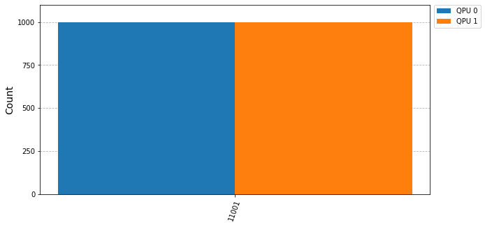
{'11001': 1000}
Time taken: 0.019545911 s.
For QPU 1, with backend BasicAer:
Result:
{'11001': 1000}
Time taken: 0.000873561 s.
First we run the circuit with the method
QPU.run(), passing the circuit, transpilation options and other run parameters. It is important to note that if we don´t specifytranspilation=True, default isFalse, therefore the user will be responsible for the tranpilation of the circuit accordingly to the native gates and topology of the backend. This method will return aqjob.QJobobject. Be aware that the key point is that theQPU.run()method is asynchronous.To get the results of the simulation, we apply the method
QJob.result(), which will return aqjob.Resultobject that stores the information in its class atributes. Depending on the simulator, we will have more or less information. Note that this is a synchronous method.Once we have the
qjob.Resultobject, we can obtain the counts dictionary byResult.get_counts(). Another method independent from the simulator isResult.time_taken(), that gives us the time of the simulation in seconds.
[5]:
%matplotlib inline

from qiskit.visualization import plot_histogram
import matplotlib.pyplot as plt
plot_histogram(counts, figsize = (10, 5), bar_labels=False, legend = [f"QPU {i}" for i in range(len(qpus))])
# plt.savefig(f"counts_{len(qpus)}_qpus.png", dpi=200)
[5]:
Cool isn’t it? But this circuit is too simple, let’s try with a more complex one!
[6]:
import json

# impoting from examples/circuits/
with open("circuits/circuit_15qubits_10layers.json", "r") as file:
    circuit = json.load(file)
We have examples of circuit in json format so you can create your own, but as we said, it is not necessary since qiskit.QuantumCircuit and OpenQASM2 are supported.
This circuit has 15 qubits and 10 intermidiate measurements, let’s run it in AerSimulator
[7]:
for qpu in qpus:
    if qpu.backend.name == "BasicAer":
        qpu0 = qpu
        break

qjob = qpu0.run(circuit, transpile = True, shots = 1000)

result = qjob.result() # bloking call

time = qjob.time_taken()

counts.append(result.get_counts())

print(f"Result: Time taken: {time} s.")
Result: Time taken: 9.131714186 s.
Takes much longer … let’s parallelize n executions in n different QPUs
Remenber that sending circuits to a given QPU is a non-blocking call, so we can use a loop, keeping the qjob.QJob objects in a list.
Then, we can wait for all the jobs to finish with the qjob.gather() function. Let’s measure time to check that we are parallelizing:
[8]:
import time
from cunqa import gather

qjobs = []
n = len(qpus)

tick = time.time()

for qpu in qpus:
    qjobs.append(qpu.run(circuit, transpile = True, shots = 1000))

results = gather(qjobs) # this is a bloking call
tack = time.time()
[9]:
print(f"Time taken to run {n} circuits in parallel: {tack - tick} s.")
print("Time for each execution:")
for i, result in enumerate(results):
    print(f"For QJob {i}, time taken: {result.time_taken} s.")
Time taken to run 2 circuits in parallel: 9.211505889892578 s.
Time for each execution:
For QJob 0, time taken: 9.059122133 s.
For QJob 1, time taken: 9.05945947 s.
Looking at the times we confirm that the circuits were run in parallel.