import os, sys

# path to access c++ files
sys.path.append(os.getenv("HOME"))

from cunqa import getQPUs

qpus  = getQPUs(local=False)

for q in qpus:
    print(f"QPU {q.id}, backend: {q.backend.name}, simulator: {q.backend.simulator}, version: {q.backend.version}.")

QPU 0, backend: SimpleSimulator, simulator: SimpleMunich, version: 0.0.1.
QPU 1, backend: SimpleSimulator, simulator: SimpleMunich, version: 0.0.1.
QPU 2, backend: SimpleSimulator, simulator: SimpleMunich, version: 0.0.1.

Examples for optimizations

Before sending a circuit to the QClient, a transpilation process occurs (if not, it is done by the user). This process, in some cases, can take much time and resources, in addition to the sending cost itself. If we were to execute a single circuit once, it shouldn´t be a big problem, but it is when it comes to variational algorithms.

This quantum-classical algorithms require several executions of the same circuit but changing the value of the parameters, which are optimized in the classical part. In order to optimize this, we developed a functionallity that allows the user to upgrade the circuit parameters with no extra transpilations of the circuit, sending to the QClient the list of the parameters ONLY. This is of much advantage to speed up the computation in the cases in which transpilation takes a significant part of the total time of the simulation.

Let´s see how to work with this feature taking as an example a Variational Quantum Algorithm for state preparation.

We start from a Hardware Efficient Ansatz to build our parametrized circuit:

from qiskit import QuantumCircuit
from qiskit.circuit import Parameter

def hardware_efficient_ansatz(num_qubits, num_layers):
    qc = QuantumCircuit(num_qubits)
    param_idx = 0
    for _ in range(num_layers):
        for qubit in range(num_qubits):
            phi = Parameter(f'phi_{param_idx}_{qubit}')
            lam = Parameter(f'lam_{param_idx}_{qubit}')
            qc.ry(phi, qubit)
            qc.rz(lam, qubit)
        param_idx += 1
        for qubit in range(num_qubits - 1):
            qc.cx(qubit, qubit + 1)
    qc.measure_all()
    return qc

The we need a cost function. We will define a target distribution and measure how far we are from it. We choose to prepare a normal distribution among all the \(2^n\) possible outcomes of the circuit.

def target_distribution(num_qubits):
    # Define a normal distribution over the states
    num_states = 2 ** num_qubits
    states = np.arange(num_states)
    mean = num_states / 2
    std_dev = num_states / 4
    target_probs = norm.pdf(states, mean, std_dev)
    target_probs /= target_probs.sum()  # Normalize to make it a valid probability distribution
    target_dist = {format(i, f'0{num_qubits}b'): target_probs[i] for i in range(num_states)}
    return target_dist

import pandas as pd
from scipy.stats import entropy, norm

def KL_divergence(counts, n_shots, target_dist):
    # Convert counts to probabilities
    pdf = pd.DataFrame.from_dict(counts, orient="index").reset_index()
    pdf.rename(columns={"index": "state", 0: "counts"}, inplace=True)
    pdf["probability"] = pdf["counts"] / n_shots

    # Create a dictionary for the obtained distribution
    obtained_dist = pdf.set_index("state")["probability"].to_dict()

    # Ensure all states are present in the obtained distribution
    for state in target_dist:
        if state not in obtained_dist:
            obtained_dist[state] = 0.0

    # Convert distributions to lists for KL divergence calculation
    target_probs = [target_dist[state] for state in sorted(target_dist)]
    obtained_probs = [obtained_dist[state] for state in sorted(obtained_dist)]

    # Calculate KL divergence
    kl_divergence = entropy(obtained_probs, target_probs)

    return kl_divergence

num_qubits = 6

num_layers = 3

n_shots = 1e5

Simply using the QPU.run() method

At first we should try the intiutive alternative: upgrading parameters at the QClient, transpiling and sending the whole circuit to the QPU.

def cost_function_run(params):
    n_shots = 1e5
    target_dist = target_distribution(num_qubits)

    circuit = ansatz.assign_parameters(params)

    result = qpu.run(circuit, transpile = True, opt_level = 0, shots = n_shots).result

    counts = result.counts

    return KL_divergence(counts, n_shots, target_dist)

Our cost function updates the parameters given by the optimizer, asigns them to the ansatz and sends the circuit with the transpilation option set True. Let´s choose a QPU to work with and go ahead with the optimization:

import numpy as np
import time

qpu = qpus[0]

ansatz = hardware_efficient_ansatz(num_qubits, num_layers)

num_parameters = ansatz.num_parameters

initial_parameters = np.zeros(num_parameters)

from scipy.optimize import minimize

i = 0

cost_run = []
individuals_run = []

def callback(xk):
    global i
    e = cost_function_run(xk)
    individuals_run.append(xk)
    cost_run.append(e)
    if i%20 == 0:
        print(f"Iteration step {i}: f(x) = {e}")
    i+=1

tick = time.time()
optimization_result_run = minimize(cost_function_run, initial_parameters, method='COBYLA',
        callback=callback, tol = 0.01,
        options={
        'disp': True,     # Print info at the end
        'maxiter': 4000   # Limit the number of iterations
    })
tack = time.time()
time_run = tack-tick
print()
print("Total optimization time: ", time_run, " s")
print()

Iteration step 0: f(x) = 5.644885693319627
Iteration step 20: f(x) = 3.2489683099416027
Iteration step 40: f(x) = 0.700518505677799
Iteration step 60: f(x) = 0.5086090832144972
Iteration step 80: f(x) = 0.43838720938090936
Iteration step 100: f(x) = 0.3712628503801477
Iteration step 120: f(x) = 0.26705681526906927
Iteration step 140: f(x) = 0.19667531489860712
Iteration step 160: f(x) = 0.1557449733702997
Iteration step 180: f(x) = 0.12627009394865418
Iteration step 200: f(x) = 0.09875260103360035
Iteration step 220: f(x) = 0.0796950348124891
Iteration step 240: f(x) = 0.08664296063303309
Iteration step 260: f(x) = 0.07786113607509895
Iteration step 280: f(x) = 0.07138004921940413
Iteration step 300: f(x) = 0.06928285629833203
Iteration step 320: f(x) = 0.06625305423998329
Iteration step 340: f(x) = 0.06791448821860378
Iteration step 360: f(x) = 0.06584292813374018
Iteration step 380: f(x) = 0.06878749095657292

   Normal return from subroutine COBYLA

   NFVALS =  391   F = 6.630927E-02    MAXCV = 0.000000E+00
   X = 2.483621E-01  -4.507945E-01   4.142488E-02   1.693378E-01   9.101863E-01
       7.824475E-02   2.095159E-01   3.357104E-01  -1.846450E-01   5.492609E-01
       6.121254E-01   5.378724E-01   6.303580E-01  -2.833794E-01  -9.201173E-02
       4.659155E-01   2.156028E-01  -1.392999E+00   8.187967E-02   4.551563E-01
       1.093445E+00   5.679521E-01   1.143250E+00   6.251608E-01   1.570452E+00
      -3.110023E-01   7.930667E-01  -3.996242E-01   8.965306E-01  -1.083956E-01
      -4.277121E-01   1.343497E+00  -7.796074E-02   1.690255E+00  -1.356059E-01
       1.691876E+00

Total optimization time:  28.403029203414917  s

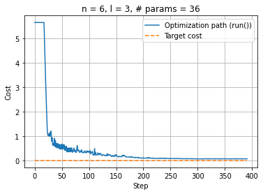
%matplotlib inline

import matplotlib.pyplot as plt
plt.clf()
plt.plot(np.linspace(0, optimization_result_run.nfev, optimization_result_run.nfev), cost_run, label="Optimization path (run())")
upper_bound = optimization_result_run.nfev
plt.plot(np.linspace(0, upper_bound, upper_bound), np.zeros(upper_bound), "--", label="Target cost")
plt.xlabel("Step"); plt.ylabel("Cost"); plt.legend(loc="upper right"); plt.title(f"n = {num_qubits}, l = {num_layers}, # params = {num_parameters}")
plt.grid(True)
plt.show()
# plt.savefig(f"optimization_run_n_{num_qubits}_p_{num_parameters}.png", dpi=200)

Using QJob.upgrade_parameters()

The first step now is to create the qjob.QJob object that which parameters we are going to upgrade in each step of the optimization; for that, we must run a circuit with initial parameters in a QPU, the procedure is as we explained above:

ansatz = hardware_efficient_ansatz(num_qubits, num_layers)

num_parameters = ansatz.num_parameters

initial_parameters = np.zeros(num_parameters)

circuit = ansatz.assign_parameters(initial_parameters)

qjob = qpu.run(circuit, transpile = True, opt_level = 0, shots = n_shots)

Now that we have sent to the virtual QPU the transpiled circuit, we can use the method qjob.QJob.upgrade_parameters() to change the rotations of the gates:

print("Result with initial_parameters: ")
print(qjob.result.counts)

random_parameters = np.random.uniform(0, 2 * np.pi, num_parameters).tolist()
print(random_parameters)
qjob.upgrade_parameters(random_parameters)

print()
print("Result with random_parameters: ")
print(qjob.result.counts)

Result with initial_parameters:
{'000000': 100000}
[4.800769084169513, 1.2169894739610545, 4.308700639089514, 0.53228562699461, 4.572801942653737, 4.101667458095368, 1.085851890521249, 1.985892017022019, 4.0998922550688555, 2.6840994154719735, 2.9905197241774086, 2.9828536502963163, 2.193155663585044, 0.5546078957132934, 4.238713832258263, 5.409654114813467, 1.6005697271722092, 0.7034015057004601, 4.371946879506468, 1.264525265909713, 4.220949121372601, 3.541658508539978, 6.122463529488255, 1.4360914785130126, 1.2467862938893313, 1.1552122896705421, 1.7255569300107159, 1.4221512402804461, 3.6973504071781655, 5.528075365251304, 0.3505244857885771, 1.8120744822423005, 0.9420785391076939, 2.6013685195652054, 5.262298544374022, 3.4664558110869947]

Result with random_parameters:
{'000000': 230, '000001': 1221, '000010': 57, '000011': 963, '000100': 1478, '000101': 2214, '000110': 2206, '000111': 126, '001000': 1082, '001001': 247, '001010': 265, '001011': 1762, '001100': 600, '001101': 235, '001110': 3517, '001111': 2204, '010000': 2878, '010001': 1813, '010010': 787, '010011': 2882, '010100': 689, '010101': 2055, '010110': 464, '010111': 1664, '011000': 466, '011001': 637, '011010': 194, '011011': 4234, '011100': 2381, '011101': 5051, '011110': 676, '011111': 1441, '100000': 1450, '100001': 721, '100010': 765, '100011': 3636, '100100': 1742, '100101': 5417, '100110': 609, '100111': 2073, '101000': 1626, '101001': 323, '101010': 120, '101011': 1520, '101100': 360, '101101': 4173, '101110': 1745, '101111': 517, '110000': 2991, '110001': 3656, '110010': 116, '110011': 202, '110100': 1315, '110101': 2523, '110110': 227, '110111': 904, '111000': 4230, '111001': 2280, '111010': 333, '111011': 1481, '111100': 111, '111101': 1333, '111110': 1267, '111111': 3515}

Important considerations:

• The method acepts parameters in a list, if you have a numpy.array, simply apply .tolist() to transform it.

• When sending the circuit and setting transpile=True, we should be carefull that the transpilation process doesn’t condense gates and combine parameters, therefore, if the user wants cunqato transpile, they must set opt_level=0.

Note that qjob.QJob.upgrade_parameters() is a non-blocking call, as it was qpu.QPU.run().

Now that we are familiar with the procedure, we can design a cost funtion that takes a set of parameters, upgrades the qjob.QJob, gets the result and calculates the divergence from the desired distribution:

def cost_function(params):
    n_shots = 100000
    target_dist = target_distribution(num_qubits)

    qjob.upgrade_parameters(params.tolist())

    counts = qjob.result.counts

    return KL_divergence(counts, n_shots, target_dist)

Now we are ready to start our optimization. We will use scipy.optimize to minimize the divergence of our result distribution from the target one:

from scipy.optimize import minimize
import time

i = 0

initial_parameters = np.zeros(num_parameters)

cost = []
individuals = []

def callback(xk):
    global i
    e = cost_function(xk)
    individuals.append(xk)
    cost.append(e)
    if i%10 == 0:
        print(f"Iteration step {i}: f(x) = {e}")
    i+=1

tick = time.time()
optimization_result = minimize(cost_function, initial_parameters, method='COBYLA',
        callback=callback, tol = 0.01,
        options={
        'disp': True,     # Print info during iterations
        'maxiter': 4000     # Limit the number of iterations
    })
tack = time.time()
time_up = tack-tick
print()
print("Total optimization time: ", time_up, " s")

Iteration step 0: f(x) = 4.808127828547751
Iteration step 10: f(x) = 3.2277447214466535
Iteration step 20: f(x) = 1.4546159328320607
Iteration step 30: f(x) = 0.8280370465217498
Iteration step 40: f(x) = 0.7268863480351391
Iteration step 50: f(x) = 0.6002777280561791
Iteration step 60: f(x) = 0.6310585988580937
Iteration step 70: f(x) = 0.531624604820937
Iteration step 80: f(x) = 0.49413409044044915
Iteration step 90: f(x) = 0.28276705189385987
Iteration step 100: f(x) = 0.28315153947896776
Iteration step 110: f(x) = 0.20441926998831558
Iteration step 120: f(x) = 0.20818472830794493
Iteration step 130: f(x) = 0.20255824135914952
Iteration step 140: f(x) = 0.17140823564605984
Iteration step 150: f(x) = 0.17354475356274046
Iteration step 160: f(x) = 0.15458380797622073
Iteration step 170: f(x) = 0.1711286646144804
Iteration step 180: f(x) = 0.18543970743296512
Iteration step 190: f(x) = 0.13357890094906225
Iteration step 200: f(x) = 0.12809092212518816
Iteration step 210: f(x) = 0.12599209681896256
Iteration step 220: f(x) = 0.10140538835702381
Iteration step 230: f(x) = 0.059547306164707076
Iteration step 240: f(x) = 0.04761332250259291
Iteration step 250: f(x) = 0.05008134672726648
Iteration step 260: f(x) = 0.053307487225548414
Iteration step 270: f(x) = 0.0460627777766594
Iteration step 280: f(x) = 0.0412203148752551
Iteration step 290: f(x) = 0.02949268274755688
Iteration step 300: f(x) = 0.029702041986933683
Iteration step 310: f(x) = 0.029368454456454612
Iteration step 320: f(x) = 0.020242468782134097
Iteration step 330: f(x) = 0.022896600154442524
Iteration step 340: f(x) = 0.02440388389920066
Iteration step 350: f(x) = 0.02136227945999611
Iteration step 360: f(x) = 0.01699669415502308
Iteration step 370: f(x) = 0.015584717555711291
Iteration step 380: f(x) = 0.014365914175310331
Iteration step 390: f(x) = 0.013330609474756292
Iteration step 400: f(x) = 0.013018092381938575
Iteration step 410: f(x) = 0.011943676000667106
Iteration step 420: f(x) = 0.012111982447111237
Iteration step 430: f(x) = 0.011964575772810473
Iteration step 440: f(x) = 0.012022413597904028
Iteration step 450: f(x) = 0.011539412823483365
Iteration step 460: f(x) = 0.011866703502954939

   Normal return from subroutine COBYLA

   NFVALS =  468   F = 1.154528E-02    MAXCV = 0.000000E+00
   X = 1.445694E+00   4.761625E-01   1.406031E+00   1.517224E+00  -4.462020E-01
       4.634130E-01   8.257513E-01   1.322178E+00   1.593436E+00  -6.847369E-02
      -1.637136E-01   3.511552E-01   1.616953E+00  -2.493556E-01   1.420238E+00
       8.484528E-01   7.009079E-01  -1.572803E-01   1.875096E+00  -1.109267E+00
       1.233791E+00   2.716658E-01   1.541790E+00   2.519028E-01   1.469977E+00
       9.737024E-01   1.623521E+00   7.760460E-01  -3.942303E-01  -5.036106E-01
       2.973732E-01   7.718844E-01  -3.806809E-01   3.187416E-01   5.901928E-01
      -8.671375E-01

Total optimization time:  29.011065244674683  s

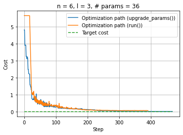
We can plot the evolution of the cost function during the optimization:

%matplotlib inline

import matplotlib.pyplot as plt
plt.clf()
plt.plot(np.linspace(0, optimization_result.nfev, optimization_result.nfev), cost, label="Optimization path (upgrade_params())")
plt.plot(np.linspace(0, optimization_result_run.nfev, optimization_result_run.nfev), cost_run, label="Optimization path (run())")
upper_bound = max(optimization_result_run.nfev, optimization_result.nfev)
plt.plot(np.linspace(0, upper_bound, upper_bound), np.zeros(upper_bound), "--", label="Target cost")
plt.xlabel("Step"); plt.ylabel("Cost"); plt.legend(loc="upper right"); plt.title(f"n = {num_qubits}, l = {num_layers}, # params = {num_parameters}")
plt.grid(True)
plt.show()
# plt.savefig(f"optimization_n_{num_qubits}_p_{num_parameters}.png", dpi=200)